Tutorial 3: Autoencoders applications
Contents
![]()

Tutorial 3: Autoencoders applications
Bonus Day: Autoencoders
By Neuromatch Academy
Content creators: Marco Brigham and the CCNSS team (2014-2018)
Content reviewers: Itzel Olivos, Karen Schroeder, Karolina Stosio, Kshitij Dwivedi, Spiros Chavlis, Michael Waskom
Production editor: Spiros Chavlis
Tutorial Objectives
Autoencoder applications
How do autoencoders with rich internal representations perform on the MNIST cognitive task?
How do autoencoders perceive unseen digit classes?
How does ANN image encoding differ from human vision?
We are equipped with tools and techniques to answer these questions, and hopefully, many others you may encounter in your research!

In this tutorial, you will:
Analyze how autoencoders perceive transformed data (added noise, occluded parts, and rotations), and how that evolves with short re-train sessions
Use autoencoders to visualize unseen digit classes
Understand visual encoding for fully connected ANN autoencoders
Setup
⚠ Experimental LLM-enhanced tutorial ⚠
This notebook includes Neuromatch’s experimental Chatify 🤖 functionality. The Chatify notebook extension adds support for a large language model-based “coding tutor” to the materials. The tutor provides automatically generated text to help explain any code cell in this notebook.
Note that using Chatify may cause breaking changes and/or provide incorrect or misleading information. If you wish to proceed by installing and enabling the Chatify extension, you should run the next two code blocks (hidden by default). If you do not want to use this experimental version of the Neuromatch materials, please use the stable materials instead.
To use the Chatify helper, insert the %%explain magic command at the start of any code cell and then run it (shift + enter) to access an interface for receiving LLM-based assitance. You can then select different options from the dropdown menus depending on what sort of assitance you want. To disable Chatify and run the code block as usual, simply delete the %%explain command and re-run the cell.
Note that, by default, all of Chatify’s responses are generated locally. This often takes several minutes per response. Once you click the “Submit request” button, just be patient– stuff is happening even if you can’t see it right away!
Thanks for giving Chatify a try! Love it? Hate it? Either way, we’d love to hear from you about your Chatify experience! Please consider filling out our brief survey to provide feedback and help us make Chatify more awesome!
Run the next two cells to install and configure Chatify…
%pip install -q davos
import davos
davos.config.suppress_stdout = True
Note: you may need to restart the kernel to use updated packages.
smuggle chatify      # pip: git+https://github.com/ContextLab/chatify.git
%load_ext chatify
Downloading and initializing model; this may take a few minutes...
llama.cpp: loading model from /home/runner/.cache/huggingface/hub/models--TheBloke--Llama-2-7B-Chat-GGML/snapshots/501a3c8182cd256a859888fff4e838c049d5d7f6/llama-2-7b-chat.ggmlv3.q5_1.bin
llama_model_load_internal: format     = ggjt v3 (latest)
llama_model_load_internal: n_vocab    = 32000
llama_model_load_internal: n_ctx      = 512
llama_model_load_internal: n_embd     = 4096
llama_model_load_internal: n_mult     = 256
llama_model_load_internal: n_head     = 32
llama_model_load_internal: n_layer    = 32
llama_model_load_internal: n_rot      = 128
llama_model_load_internal: freq_base  = 10000.0
llama_model_load_internal: freq_scale = 1
llama_model_load_internal: ftype      = 9 (mostly Q5_1)
llama_model_load_internal: n_ff       = 11008
llama_model_load_internal: model size = 7B
llama_model_load_internal: ggml ctx size =    0.08 MB
llama_model_load_internal: mem required  = 6390.60 MB (+ 1026.00 MB per state)
AVX = 1 | AVX2 = 1 | AVX512 = 1 | AVX512_VBMI = 0 | AVX512_VNNI = 0 | FMA = 1 | NEON = 0 | ARM_FMA = 0 | F16C = 1 | FP16_VA = 0 | WASM_SIMD = 0 | BLAS = 0 | SSE3 = 1 | VSX = 0 | llama_new_context_with_model: kv self size = 256.00 MB
Install and import feedback gadget
# @title Install and import feedback gadget

!pip3 install vibecheck datatops --quiet

from vibecheck import DatatopsContentReviewContainer
def content_review(notebook_section: str):
    return DatatopsContentReviewContainer(
        "",  # No text prompt
        notebook_section,
        {
            "url": "https://pmyvdlilci.execute-api.us-east-1.amazonaws.com/klab",
            "name": "neuromatch_cn",
            "user_key": "y1x3mpx5",
        },
    ).render()


feedback_prefix = "Bonus_Autoencoders_T3"
# Imports
import numpy as np
import matplotlib.pyplot as plt
import os
from scipy import ndimage

import torch
from torch import nn, optim

from sklearn.datasets import fetch_openml
Figure settings
# @title Figure settings
import logging
logging.getLogger('matplotlib.font_manager').disabled = True
%config InlineBackend.figure_format = 'retina'
plt.style.use("https://raw.githubusercontent.com/NeuromatchAcademy/course-content/NMA2020/nma.mplstyle")
Helper functions
# @title Helper functions
def downloadMNIST():
"""
Download MNIST dataset and transform it to torch.Tensor
Args:
None
Returns:
x_train : training images (torch.Tensor) (60000, 28, 28)
x_test : test images (torch.Tensor) (10000, 28, 28)
y_train : training labels (torch.Tensor) (60000, )
y_train : test labels (torch.Tensor) (10000, )
"""
X, y = fetch_openml('mnist_784', version=1, return_X_y=True, as_frame=False)
# Trunk the data
n_train = 60000
n_test = 10000
train_idx = np.arange(0, n_train)
test_idx = np.arange(n_train, n_train + n_test)
x_train, y_train = X[train_idx], y[train_idx]
x_test, y_test = X[test_idx], y[test_idx]
# Transform np.ndarrays to torch.Tensor
x_train = torch.from_numpy(np.reshape(x_train,
(len(x_train),
28, 28)).astype(np.float32))
x_test = torch.from_numpy(np.reshape(x_test,
(len(x_test),
28, 28)).astype(np.float32))
y_train = torch.from_numpy(y_train.astype(int))
y_test = torch.from_numpy(y_test.astype(int))
return (x_train, y_train, x_test, y_test)
def init_weights_kaiming_uniform(layer):
"""
Initializes weights from linear PyTorch layer
with kaiming uniform distribution.
Args:
layer (torch.Module)
Pytorch layer
Returns:
Nothing.
"""
# check for linear PyTorch layer
if isinstance(layer, nn.Linear):
# initialize weights with kaiming uniform distribution
nn.init.kaiming_uniform_(layer.weight.data)
def init_weights_kaiming_normal(layer):
"""
Initializes weights from linear PyTorch layer
with kaiming normal distribution.
Args:
layer (torch.Module)
Pytorch layer
Returns:
Nothing.
"""
# check for linear PyTorch layer
if isinstance(layer, nn.Linear):
# initialize weights with kaiming normal distribution
nn.init.kaiming_normal_(layer.weight.data)
def get_layer_weights(layer):
"""
Retrieves learnable parameters from PyTorch layer.
Args:
layer (torch.Module)
Pytorch layer
Returns:
list with learnable parameters
"""
# initialize output list
weights = []
# check whether layer has learnable parameters
if layer.parameters():
# copy numpy array representation of each set of learnable parameters
for item in layer.parameters():
weights.append(item.detach().numpy())
return weights
def eval_mse(y_pred, y_true):
"""
Evaluates mean square error (MSE) between y_pred and y_true
Args:
y_pred (torch.Tensor)
prediction samples
v (numpy array of floats)
ground truth samples
Returns:
MSE(y_pred, y_true)
"""
with torch.no_grad():
criterion = nn.MSELoss()
loss = criterion(y_pred, y_true)
return float(loss)
def eval_bce(y_pred, y_true):
"""
Evaluates binary cross-entropy (BCE) between y_pred and y_true
Args:
y_pred (torch.Tensor)
prediction samples
v (numpy array of floats)
ground truth samples
Returns:
BCE(y_pred, y_true)
"""
with torch.no_grad():
criterion = nn.BCELoss()
loss = criterion(y_pred, y_true)
return float(loss)
def plot_row(images, show_n=10, image_shape=None):
"""
Plots rows of images from list of iterables (iterables: list, numpy array
or torch.Tensor). Also accepts single iterable.
Randomly selects images in each list element if item count > show_n.
Args:
images (iterable or list of iterables)
single iterable with images, or list of iterables
show_n (integer)
maximum number of images per row
image_shape (tuple or list)
original shape of image if vectorized form
Returns:
Nothing.
"""
if not isinstance(images, (list, tuple)):
images = [images]
for items_idx, items in enumerate(images):
items = np.array(items)
if items.ndim == 1:
items = np.expand_dims(items, axis=0)
if len(items) > show_n:
selected = np.random.choice(len(items), show_n, replace=False)
items = items[selected]
if image_shape is not None:
items = items.reshape([-1] + list(image_shape))
plt.figure(figsize=(len(items) * 1.5, 2))
for image_idx, image in enumerate(items):
plt.subplot(1, len(items), image_idx + 1)
plt.imshow(image, cmap='gray', vmin=image.min(), vmax=image.max())
plt.axis('off')
plt.tight_layout()
def to_s2(u):
"""
Projects 3D coordinates to spherical coordinates (theta, phi) surface of
unit sphere S2.
theta: [0, pi]
phi: [-pi, pi]
Args:
u (list, numpy array or torch.Tensor of floats)
3D coordinates
Returns:
Sperical coordinates (theta, phi) on surface of unit sphere S2.
"""
x, y, z = (u[:, 0], u[:, 1], u[:, 2])
r = np.sqrt(x**2 + y**2 + z**2)
theta = np.arccos(z / r)
phi = np.arctan2(x, y)
return np.array([theta, phi]).T
def to_u3(s):
"""
Converts from 2D coordinates on surface of unit sphere S2 to 3D coordinates
(on surface of S2), i.e. (theta, phi) ---> (1, theta, phi).
Args:
s (list, numpy array or torch.Tensor of floats)
2D coordinates on unit sphere S_2
Returns:
3D coordinates on surface of unit sphere S_2
"""
theta, phi = (s[:, 0], s[:, 1])
x = np.sin(theta) * np.sin(phi)
y = np.sin(theta) * np.cos(phi)
z = np.cos(theta)
return np.array([x, y, z]).T
def xy_lim(x):
"""
Return arguments for plt.xlim and plt.ylim calculated from minimum
and maximum of x.
Args:
x (list, numpy array or torch.Tensor of floats)
data to be plotted
Returns:
Nothing.
"""
x_min = np.min(x, axis=0)
x_max = np.max(x, axis=0)
x_min = x_min - np.abs(x_max - x_min) * 0.05 - np.finfo(float).eps
x_max = x_max + np.abs(x_max - x_min) * 0.05 + np.finfo(float).eps
return [x_min[0], x_max[0]], [x_min[1], x_max[1]]
def plot_generative(x, decoder_fn, image_shape, n_row=16, s2=False):
"""
Plots images reconstructed by decoder_fn from a 2D grid in
latent space that is determined by minimum and maximum values in x.
Args:
x (list, numpy array or torch.Tensor of floats)
2D or 3D coordinates in latent space
decoder_fn (integer)
function returning vectorized images from 2D latent space coordinates
image_shape (tuple or list)
original shape of image
n_row (integer)
number of rows in grid
s2 (boolean)
convert 3D coordinates (x, y, z) to spherical coordinates (theta, phi)
Returns:
Nothing.
"""
if s2:
x = to_s2(np.array(x))
xlim, ylim = xy_lim(np.array(x))
dx = (xlim[1] - xlim[0]) / n_row
grid = [np.linspace(ylim[0] + dx / 2, ylim[1] - dx / 2, n_row),
np.linspace(xlim[0] + dx / 2, xlim[1] - dx / 2, n_row)]
canvas = np.zeros((image_shape[0] * n_row, image_shape[1] * n_row))
cmap = plt.get_cmap('gray')
for j, latent_y in enumerate(grid[0][::-1]):
for i, latent_x in enumerate(grid[1]):
latent = np.array([[latent_x, latent_y]], dtype=np.float32)
if s2:
latent = to_u3(latent)
with torch.no_grad():
x_decoded = decoder_fn(torch.from_numpy(latent))
x_decoded = x_decoded.reshape(image_shape)
canvas[j * image_shape[0]: (j + 1) * image_shape[0],
i * image_shape[1]: (i + 1) * image_shape[1]] = x_decoded
plt.imshow(canvas, cmap=cmap, vmin=canvas.min(), vmax=canvas.max())
plt.axis('off')
def plot_latent(x, y, show_n=500, s2=False, fontdict=None, xy_labels=None):
"""
Plots digit class of each sample in 2D latent space coordinates.
Args:
x (list, numpy array or torch.Tensor of floats)
2D coordinates in latent space
y (list, numpy array or torch.Tensor of floats)
digit class of each sample
n_row (integer)
number of samples
s2 (boolean)
convert 3D coordinates (x, y, z) to spherical coordinates (theta, phi)
fontdict (dictionary)
style option for plt.text
xy_labels (list)
optional list with [xlabel, ylabel]
Returns:
Nothing.
"""
if fontdict is None:
fontdict = {'weight': 'bold', 'size': 12}
if s2:
x = to_s2(np.array(x))
cmap = plt.get_cmap('tab10')
if len(x) > show_n:
selected = np.random.choice(len(x), show_n, replace=False)
x = x[selected]
y = y[selected]
for my_x, my_y in zip(x, y):
plt.text(my_x[0], my_x[1], str(int(my_y)),
color=cmap(int(my_y) / 10.),
fontdict=fontdict,
horizontalalignment='center',
verticalalignment='center',
alpha=0.8)
xlim, ylim = xy_lim(np.array(x))
plt.xlim(xlim)
plt.ylim(ylim)
if s2:
if xy_labels is None:
xy_labels = [r'$\varphi$', r'$\theta$']
plt.xticks(np.arange(0, np.pi + np.pi / 6, np.pi / 6),
['0', '$\pi/6$', '$\pi/3$', '$\pi/2$',
'$2\pi/3$', '$5\pi/6$', '$\pi$'])
plt.yticks(np.arange(-np.pi, np.pi + np.pi / 3, np.pi / 3),
['$-\pi$', '$-2\pi/3$', '$-\pi/3$', '0',
'$\pi/3$', '$2\pi/3$', '$\pi$'])
if xy_labels is None:
xy_labels = ['$Z_1$', '$Z_2$']
plt.xlabel(xy_labels[0])
plt.ylabel(xy_labels[1])
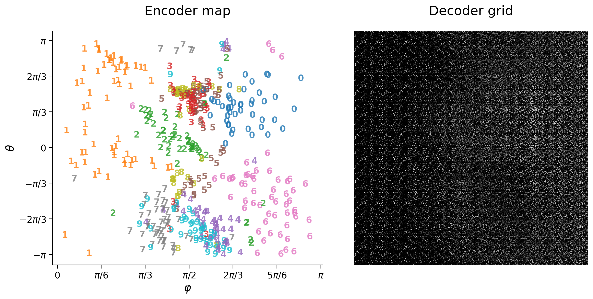
def plot_latent_generative(x, y, decoder_fn, image_shape, s2=False,
title=None, xy_labels=None):
"""
Two horizontal subplots generated with encoder map and decoder grid.
Args:
x (list, numpy array or torch.Tensor of floats)
2D coordinates in latent space
y (list, numpy array or torch.Tensor of floats)
digit class of each sample
decoder_fn (integer)
function returning vectorized images from 2D latent space coordinates
image_shape (tuple or list)
original shape of image
s2 (boolean)
convert 3D coordinates (x, y, z) to spherical coordinates (theta, phi)
title (string)
plot title
xy_labels (list)
optional list with [xlabel, ylabel]
Returns:
Nothing.
"""
fig = plt.figure(figsize=(12, 6))
if title is not None:
fig.suptitle(title, y=1.05)
ax = fig.add_subplot(121)
ax.set_title('Encoder map', y=1.05)
plot_latent(x, y, s2=s2, xy_labels=xy_labels)
ax = fig.add_subplot(122)
ax.set_title('Decoder grid', y=1.05)
plot_generative(x, decoder_fn, image_shape, s2=s2)
plt.tight_layout()
plt.show()
def plot_latent_ab(x1, x2, y, selected_idx=None,
title_a='Before', title_b='After', show_n=500, s2=False):
"""
Two horizontal subplots with encoder maps.
Args:
x1 (list, numpy array or torch.Tensor of floats)
2D coordinates in latent space (left plot)
x2 (list, numpy array or torch.Tensor of floats)
digit class of each sample (right plot)
y (list, numpy array or torch.Tensor of floats)
digit class of each sample
selected_idx (list of integers)
indexes of elements to be plotted
show_n (integer)
maximum number of samples in each plot
s2 (boolean)
convert 3D coordinates (x, y, z) to spherical coordinates (theta, phi)
Returns:
Nothing.
"""
fontdict = {'weight': 'bold', 'size': 12}
if len(x1) > show_n:
if selected_idx is None:
selected_idx = np.random.choice(len(x1), show_n, replace=False)
x1 = x1[selected_idx]
x2 = x2[selected_idx]
y = y[selected_idx]
data = np.concatenate([x1, x2])
if s2:
xlim, ylim = xy_lim(to_s2(data))
else:
xlim, ylim = xy_lim(data)
plt.figure(figsize=(12, 6))
ax = plt.subplot(121)
ax.set_title(title_a, y=1.05)
plot_latent(x1, y, fontdict=fontdict, s2=s2)
plt.xlim(xlim)
plt.ylim(ylim)
ax = plt.subplot(122)
ax.set_title(title_b, y=1.05)
plot_latent(x2, y, fontdict=fontdict, s2=s2)
plt.xlim(xlim)
plt.ylim(ylim)
plt.tight_layout()
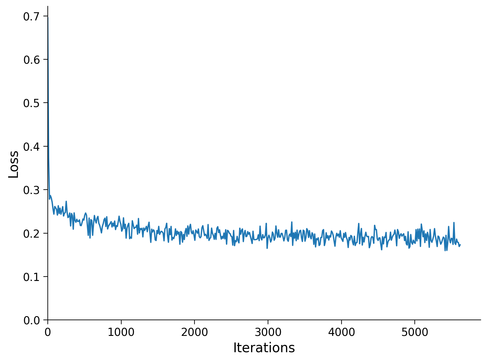
def runSGD(net, input_train, input_test, out_train=None, out_test=None,
optimizer=None, criterion='bce', n_epochs=10, batch_size=32,
verbose=False):
"""
Trains autoencoder network with stochastic gradient descent with
optimizer and loss criterion. Train samples are shuffled, and loss is
displayed at the end of each opoch for both MSE and BCE. Plots training loss
at each minibatch (maximum of 500 randomly selected values).
Args:
net (torch network)
ANN network (nn.Module)
input_train (torch.Tensor)
vectorized input images from train set
input_test (torch.Tensor)
vectorized input images from test set
criterion (string)
train loss: 'bce' or 'mse'
out_train (torch.Tensor)
optional target images from train set
out_test (torch.Tensor)
optional target images from test set
optimizer (torch optimizer)
optional target images from train set
criterion (string)
train loss: 'bce' or 'mse'
n_epochs (boolean)
number of full iterations of training data
batch_size (integer)
number of element in mini-batches
verbose (boolean)
whether to print final loss
Returns:
Nothing.
"""
if out_train is not None and out_test is not None:
different_output = True
else:
different_output = False
# Initialize loss function
if criterion == 'mse':
loss_fn = nn.MSELoss()
elif criterion == 'bce':
loss_fn = nn.BCELoss()
else:
print('Please specify either "mse" or "bce" for loss criterion')
# Initialize SGD optimizer
if optimizer is None:
optimizer = optim.Adam(net.parameters())
# Placeholder for loss
track_loss = []
print('Epoch', '\t', 'Loss train', '\t', 'Loss test')
for i in range(n_epochs):
shuffle_idx = np.random.permutation(len(input_train))
batches = torch.split(input_train[shuffle_idx], batch_size)
if different_output:
batches_out = torch.split(out_train[shuffle_idx], batch_size)
for batch_idx, batch in enumerate(batches):
output_train = net(batch)
if different_output:
loss = loss_fn(output_train, batches_out[batch_idx])
else:
loss = loss_fn(output_train, batch)
optimizer.zero_grad()
loss.backward()
optimizer.step()
# Keep track of loss at each epoch
track_loss += [float(loss)]
loss_epoch = f'{i+1}/{n_epochs}'
with torch.no_grad():
output_train = net(input_train)
if different_output:
loss_train = loss_fn(output_train, out_train)
else:
loss_train = loss_fn(output_train, input_train)
loss_epoch += f'\t {loss_train:.4f}'
output_test = net(input_test)
if different_output:
loss_test = loss_fn(output_test, out_test)
else:
loss_test = loss_fn(output_test, input_test)
loss_epoch += f'\t\t {loss_test:.4f}'
print(loss_epoch)
if verbose:
# Print loss
if different_output:
loss_mse = f'\nMSE\t {eval_mse(output_train, out_train):0.4f}'
loss_mse += f'\t\t {eval_mse(output_test, out_test):0.4f}'
else:
loss_mse = f'\nMSE\t {eval_mse(output_train, input_train):0.4f}'
loss_mse += f'\t\t {eval_mse(output_test, input_test):0.4f}'
print(loss_mse)
if different_output:
loss_bce = f'BCE\t {eval_bce(output_train, out_train):0.4f}'
loss_bce += f'\t\t {eval_bce(output_test, out_test):0.4f}'
else:
loss_bce = f'BCE\t {eval_bce(output_train, input_train):0.4f}'
loss_bce += f'\t\t {eval_bce(output_test, input_test):0.4f}'
print(loss_bce)
# Plot loss
step = int(np.ceil(len(track_loss)/500))
x_range = np.arange(0, len(track_loss), step)
plt.figure()
plt.plot(x_range, track_loss[::step], 'C0')
plt.xlabel('Iterations')
plt.ylabel('Loss')
plt.xlim([0, None])
plt.ylim([0, None])
plt.show()
def image_occlusion(x, image_shape):
"""
Randomly selects on quadrant of images and sets to zeros.
Args:
x (torch.Tensor of floats)
vectorized images
image_shape (tuple or list)
original shape of image
Returns:
torch.Tensor.
"""
selection = np.random.choice(4, len(x))
my_x = np.array(x).copy()
my_x = my_x.reshape(-1, image_shape[0], image_shape[1])
my_x[selection == 0, :int(image_shape[0] / 2), :int(image_shape[1] / 2)] = 0
my_x[selection == 1, int(image_shape[0] / 2):, :int(image_shape[1] / 2)] = 0
my_x[selection == 2, :int(image_shape[0] / 2), int(image_shape[1] / 2):] = 0
my_x[selection == 3, int(image_shape[0] / 2):, int(image_shape[1] / 2):] = 0
my_x = my_x.reshape(x.shape)
return torch.from_numpy(my_x)
def image_rotation(x, deg, image_shape):
"""
Randomly rotates images by +- deg degrees.
Args:
x (torch.Tensor of floats)
vectorized images
deg (integer)
rotation range
image_shape (tuple or list)
original shape of image
Returns:
torch.Tensor.
"""
my_x = np.array(x).copy()
my_x = my_x.reshape(-1, image_shape[0], image_shape[1])
for idx, item in enumerate(my_x):
my_deg = deg * 2 * np.random.random() - deg
my_x[idx] = ndimage.rotate(my_x[idx], my_deg,
reshape=False, prefilter=False)
my_x = my_x.reshape(x.shape)
return torch.from_numpy(my_x)
class AutoencoderClass(nn.Module):
"""
Deep autoencoder network object (nn.Module) with optional L2 normalization
of activations in bottleneck layer.
Args:
input_size (integer)
size of input samples
s2 (boolean)
whether to L2 normalize activatinos in bottleneck layer
Returns:
Autoencoder object inherited from nn.Module class.
"""
def __init__(self, input_size=784, s2=False):
super().__init__()
self.input_size = input_size
self.s2 = s2
if s2:
self.encoding_size = 3
else:
self.encoding_size = 2
self.enc1 = nn.Linear(self.input_size, int(self.input_size / 2))
self.enc1_f = nn.PReLU()
self.enc2 = nn.Linear(int(self.input_size / 2), self.encoding_size * 32)
self.enc2_f = nn.PReLU()
self.enc3 = nn.Linear(self.encoding_size * 32, self.encoding_size)
self.enc3_f = nn.PReLU()
self.dec1 = nn.Linear(self.encoding_size, self.encoding_size * 32)
self.dec1_f = nn.PReLU()
self.dec2 = nn.Linear(self.encoding_size * 32, int(self.input_size / 2))
self.dec2_f = nn.PReLU()
self.dec3 = nn.Linear(int(self.input_size / 2), self.input_size)
self.dec3_f = nn.Sigmoid()
def encoder(self, x):
"""
Encoder component.
"""
x = self.enc1_f(self.enc1(x))
x = self.enc2_f(self.enc2(x))
x = self.enc3_f(self.enc3(x))
if self.s2:
x = nn.functional.normalize(x, p=2, dim=1)
return x
def decoder(self, x):
"""
Decoder component.
"""
x = self.dec1_f(self.dec1(x))
x = self.dec2_f(self.dec2(x))
x = self.dec3_f(self.dec3(x))
return x
def forward(self, x):
"""
Forward pass.
"""
x = self.encoder(x)
x = self.decoder(x)
return x
def save_checkpoint(net, optimizer, filename):
"""
Saves a PyTorch checkpoint.
Args:
net (torch network)
ANN network (nn.Module)
optimizer (torch optimizer)
optimizer for SGD
filename (string)
filename (without extension)
Returns:
Nothing.
"""
torch.save({'model_state_dict': net.state_dict(),
'optimizer_state_dict': optimizer.state_dict()},
filename+'.pt')
def load_checkpoint(url, filename):
"""
Loads a PyTorch checkpoint from URL is local file not present.
Args:
url (string)
URL location of PyTorch checkpoint
filename (string)
filename (without extension)
Returns:
PyTorch checkpoint of saved model.
"""
if not os.path.isfile(filename+'.pt'):
os.system(f"wget {url}.pt")
return torch.load(filename+'.pt')
def reset_checkpoint(net, optimizer, checkpoint):
"""
Resets PyTorch model to checkpoint.
Args:
net (torch network)
ANN network (nn.Module)
optimizer (torch optimizer)
optimizer for SGD
checkpoint (torch checkpoint)
checkpoint of saved model
Returns:
Nothing.
"""
net.load_state_dict(checkpoint['model_state_dict'])
optimizer.load_state_dict(checkpoint['optimizer_state_dict'])
Section 0: introduction
Video 1: Applications
Submit your feedback
# @title Submit your feedback
content_review(f"{feedback_prefix}_Applications_Video")
Section 1: Download and prepare MNIST dataset
We use the helper function downloadMNIST to download the dataset and transform it into torch.Tensor and assign train and test sets to (x_train, y_train) and (x_test, y_test).
The variable input_size stores the length of vectorized versions of the images input_train and input_test for training and test images.
Instructions:
Please execute the cell below
# Download MNIST
x_train, y_train, x_test, y_test = downloadMNIST()

x_train = x_train / 255
x_test = x_test / 255

image_shape = x_train.shape[1:]

input_size = np.prod(image_shape)

input_train = x_train.reshape([-1, input_size])
input_test = x_test.reshape([-1, input_size])

test_selected_idx = np.random.choice(len(x_test), 10, replace=False)
train_selected_idx = np.random.choice(len(x_train), 10, replace=False)

test_subset_idx = np.random.choice(len(x_test), 500, replace=False)

print(f'shape image \t\t {image_shape}')
print(f'shape input_train \t {input_train.shape}')
print(f'shape input_test \t {input_test.shape}')
/opt/hostedtoolcache/Python/3.9.17/x64/lib/python3.9/site-packages/sklearn/datasets/_openml.py:1002: FutureWarning: The default value of `parser` will change from `'liac-arff'` to `'auto'` in 1.4. You can set `parser='auto'` to silence this warning. Therefore, an `ImportError` will be raised from 1.4 if the dataset is dense and pandas is not installed. Note that the pandas parser may return different data types. See the Notes Section in fetch_openml's API doc for details.
  warn(
shape image 		 torch.Size([28, 28])
shape input_train 	 torch.Size([60000, 784])
shape input_test 	 torch.Size([10000, 784])
Section 2: Download a pre-trained model
The class AutoencoderClass implements the autoencoder architectures introduced in the previous tutorial. The design of this class follows the object-oriented programming (OOP) style from tutorial W3D4. Setting the boolean parameter s2=True specifies the model with projection onto the \(S_2\) sphere.
We trained both models for n_epochs=25 and saved the weights to avoid a lengthy initial training period - these will be our reference model states.
Experiments are run from the identical initial conditions by resetting the autoencoder to the reference state at the beginning of each exercise.
The mechanism for loading and storing models from PyTorch is the following:
model = nn.Sequential(...)
or
model = AutoencoderClass()
and then
torch.save({'model_state_dict': model.state_dict(),
            'optimizer_state_dict': optimizer.state_dict()},
           filename_path)

checkpoint = torch.load(filename_path)

model.load_state_dict(checkpoint['model_state_dict'])
optimizer.load_state_dict(checkpoint['optimizer_state_dict'])
See additional PyTorch instructions, and when to use model.eval() and model.train() for more complex models.
We provide the functions save_checkpoint, load_checkpoint, and reset_checkpoint to implement the steps above and download pre-trained weights from the GitHub repo.
If downloading from GitHub fails, please uncomment the 3rd cell bellow to train the model for n_epochs=10 and save it locally.
Instructions:
Please execute the cell(s) below
root = 'https://github.com/mpbrigham/colaboratory-figures/raw/master/nma/autoencoders'
filename = 'ae_6h_prelu_bce_adam_25e_32b'
url = os.path.join(root, filename)
s2 = True

if s2:
  filename += '_s2'
  url += '_s2'
model = AutoencoderClass(s2=s2)
optimizer = optim.Adam(model.parameters())

encoder = model.encoder
decoder = model.decoder

checkpoint = load_checkpoint(url, filename)

model.load_state_dict(checkpoint['model_state_dict'])
optimizer.load_state_dict(checkpoint['optimizer_state_dict'])
--2023-07-23 19:04:35--  https://github.com/mpbrigham/colaboratory-figures/raw/master/nma/autoencoders/ae_6h_prelu_bce_adam_25e_32b_s2.pt
Resolving github.com (github.com)... 192.30.255.113
Connecting to github.com (github.com)|192.30.255.113|:443... connected.
HTTP request sent, awaiting response...
302 Found
Location: https://raw.githubusercontent.com/mpbrigham/colaboratory-figures/master/nma/autoencoders/ae_6h_prelu_bce_adam_25e_32b_s2.pt [following]
--2023-07-23 19:04:35--  https://raw.githubusercontent.com/mpbrigham/colaboratory-figures/master/nma/autoencoders/ae_6h_prelu_bce_adam_25e_32b_s2.pt
Resolving raw.githubusercontent.com (raw.githubusercontent.com)... 185.199.110.133, 185.199.108.133, 185.199.109.133, ...
Connecting to raw.githubusercontent.com (raw.githubusercontent.com)|185.199.110.133|:443... connected.
HTTP request sent, awaiting response...
200 OK
Length: 8313616 (7.9M) [application/octet-stream]
Saving to: ‘ae_6h_prelu_bce_adam_25e_32b_s2.pt’

     0K .......... .......... .......... .......... ..........  0% 99.0M 0s
    50K .......... .......... .......... .......... ..........  1% 44.4M 0s
   100K .......... .......... .......... .......... ..........  1% 47.9M 0s
   150K .......... .......... .......... .......... ..........  2%  154M 0s
   200K .......... .......... .......... .......... ..........  3% 94.6M 0s
   250K .......... .......... .......... .......... ..........  3% 38.3M 0s
   300K .......... .......... .......... .......... ..........  4% 93.6M 0s
   350K .......... .......... .......... .......... ..........  4% 92.1M 0s
   400K .......... .......... .......... .......... ..........  5%  101M 0s
   450K .......... .......... .......... .......... ..........  6%  114M 0s
   500K .......... .......... .......... .......... ..........  6%  261M 0s
   550K .......... .......... .......... .......... ..........  7%  137M 0s
   600K .......... .......... .......... .......... ..........  8%  246M 0s
   650K .......... .......... .......... .......... ..........  8%  161M 0s
   700K .......... .......... .......... .......... ..........  9%  226M 0s
   750K .......... .......... .......... .......... ..........  9%  266M 0s
   800K .......... .......... .......... .......... .......... 10%  163M 0s
   850K .......... .......... .......... .......... .......... 11%  179M 0s
   900K .......... .......... .......... .......... .......... 11%  193M 0s
   950K .......... .......... .......... .......... .......... 12%  271M 0s
  1000K .......... .......... .......... .......... .......... 12%  141M 0s
  1050K .......... .......... .......... .......... .......... 13%  240M 0s
  1100K .......... .......... .......... .......... .......... 14%  301M 0s
  1150K .......... .......... .......... .......... .......... 14%  155M 0s
  1200K .......... .......... .......... .......... .......... 15%  212M 0s
  1250K .......... .......... .......... .......... .......... 16%  149M 0s
  1300K .......... .......... .......... .......... .......... 16%  216M 0s
  1350K .......... .......... .......... .......... .......... 17%  169M 0s
  1400K .......... .......... .......... .......... .......... 17%  239M 0s
  1450K .......... .......... .......... .......... .......... 18%  166M 0s
  1500K .......... .......... .......... .......... .......... 19%  258M 0s
  1550K .......... .......... .......... .......... .......... 19%  285M 0s
  1600K .......... .......... .......... .......... .......... 20%  155M 0s
  1650K .......... .......... .......... .......... .......... 20%  242M 0s
  1700K .......... .......... .......... .......... .......... 21%  173M 0s
  1750K .......... .......... .......... .......... .......... 22%  290M 0s
  1800K .......... .......... .......... .......... .......... 22%  241M 0s
  1850K .......... .......... .......... .......... .......... 23%  252M 0s
  1900K .......... .......... .......... .......... .......... 24%  135M 0s
  1950K .......... .......... .......... .......... .......... 24%  306M 0s
  2000K .......... .......... .......... .......... .......... 25%  153M 0s
  2050K .......... .......... .......... .......... .......... 25%  218M 0s
  2100K .......... .......... .......... .......... .......... 26%  138M 0s
  2150K .......... .......... .......... .......... .......... 27%  254M 0s
  2200K .......... .......... .......... .......... .......... 27%  213M 0s
  2250K .......... .......... .......... .......... .......... 28%  206M 0s
  2300K .......... .......... .......... .......... .......... 28%  293M 0s
  2350K .......... .......... .......... .......... .......... 29%  210M 0s
  2400K .......... .......... .......... .......... .......... 30%  304M 0s
  2450K .......... .......... .......... .......... .......... 30%  143M 0s
  2500K .......... .......... .......... .......... .......... 31%  290M 0s
  2550K .......... .......... .......... .......... .......... 32%  151M 0s
  2600K .......... .......... .......... .......... .......... 32%  292M 0s
  2650K .......... .......... .......... .......... .......... 33%  226M 0s
  2700K .......... .......... .......... .......... .......... 33%  287M 0s
  2750K .......... .......... .......... .......... .......... 34%  154M 0s
  2800K .......... .......... .......... .......... .......... 35%  195M 0s
  2850K .......... .......... .......... .......... .......... 35%  112M 0s
  2900K .......... .......... .......... .......... .......... 36%  285M 0s
  2950K .......... .......... .......... .......... .......... 36%  294M 0s
  3000K .......... .......... .......... .......... .......... 37%  121M 0s
  3050K .......... .......... .......... .......... .......... 38%  247M 0s
  3100K .......... .......... .......... .......... .......... 38%  303M 0s
  3150K .......... .......... .......... .......... .......... 39%  297M 0s
  3200K .......... .......... .......... .......... .......... 40%  302M 0s
  3250K .......... .......... .......... .......... .......... 40%  249M 0s
  3300K .......... .......... .......... .......... .......... 41%  208M 0s
  3350K .......... .......... .......... .......... .......... 41%  220M 0s
  3400K .......... .......... .......... .......... .......... 42%  275M 0s
  3450K .......... .......... .......... .......... .......... 43%  161M 0s
  3500K .......... .......... .......... .......... .......... 43%  242M 0s
  3550K .......... .......... .......... .......... .......... 44%  298M 0s
  3600K .......... .......... .......... .......... .......... 44%  170M 0s
  3650K .......... .......... .......... .......... .......... 45%  225M 0s
  3700K .......... .......... .......... .......... .......... 46%  297M 0s
  3750K .......... .......... .......... .......... .......... 46%  239M 0s
  3800K .......... .......... .......... .......... .......... 47%  269M 0s
  3850K .......... .......... .......... .......... .......... 48%  249M 0s
  3900K .......... .......... .......... .......... .......... 48%  157M 0s
  3950K .......... .......... .......... .......... .......... 49%  272M 0s
  4000K .......... .......... .......... .......... .......... 49%  240M 0s
  4050K .......... .......... .......... .......... .......... 50%  248M 0s
  4100K .......... .......... .......... .......... .......... 51%  150M 0s
  4150K .......... .......... .......... .......... .......... 51%  188M 0s
  4200K .......... .......... .......... .......... .......... 52%  211M 0s
  4250K .......... .......... .......... .......... .......... 52%  257M 0s
  4300K .......... .......... .......... .......... .......... 53%  296M 0s
  4350K .......... .......... .......... .......... .......... 54%  160M 0s
  4400K .......... .......... .......... .......... .......... 54%  230M 0s
  4450K .......... .......... .......... .......... .......... 55%  246M 0s
  4500K .......... .......... .......... .......... .......... 56%  212M 0s
  4550K .......... .......... .......... .......... .......... 56%  217M 0s
  4600K .......... .......... .......... .......... .......... 57%  218M 0s
  4650K .......... .......... .......... .......... .......... 57%  194M 0s
  4700K .......... .......... .......... .......... .......... 58%  188M 0s
  4750K .......... .......... .......... .......... .......... 59%  280M 0s
  4800K .......... .......... .......... .......... .......... 59%  284M 0s
  4850K .......... .......... .......... .......... .......... 60%  140M 0s
  4900K .......... .......... .......... .......... .......... 60%  280M 0s
  4950K .......... .......... .......... .......... .......... 61%  176M 0s
  5000K .......... .......... .......... .......... .......... 62%  272M 0s
  5050K .......... .......... .......... .......... .......... 62%  149M 0s
  5100K .......... .......... .......... .......... .......... 63%  272M 0s
  5150K .......... .......... .......... .......... .......... 64%  277M 0s
  5200K .......... .......... .......... .......... .......... 64%  252M 0s
  5250K .......... .......... .......... .......... .......... 65% 96.0M 0s
  5300K .......... .......... .......... .......... .......... 65%  267M 0s
  5350K .......... .......... .......... .......... .......... 66%  287M 0s
  5400K .......... .......... .......... .......... .......... 67%  149M 0s
  5450K .......... .......... .......... .......... .......... 67%  240M 0s
  5500K .......... .......... .......... .......... .......... 68%  245M 0s
  5550K .......... .......... .......... .......... .......... 68%  287M 0s
  5600K .......... .......... .......... .......... .......... 69%  154M 0s
  5650K .......... .......... .......... .......... .......... 70%  171M 0s
  5700K .......... .......... .......... .......... .......... 70%  187M 0s
  5750K .......... .......... .......... .......... .......... 71%  281M 0s
  5800K .......... .......... .......... .......... .......... 72%  285M 0s
  5850K .......... .......... .......... .......... .......... 72%  254M 0s
  5900K .......... .......... .......... .......... .......... 73%  261M 0s
  5950K .......... .......... .......... .......... .......... 73%  228M 0s
  6000K .......... .......... .......... .......... .......... 74%  297M 0s
  6050K .......... .......... .......... .......... .......... 75%  173M 0s
  6100K .......... .......... .......... .......... .......... 75%  294M 0s
  6150K .......... .......... .......... .......... .......... 76%  178M 0s
  6200K .......... .......... .......... .......... .......... 76%  294M 0s
  6250K .......... .......... .......... .......... .......... 77%  157M 0s
  6300K .......... .......... .......... .......... .......... 78%  267M 0s
  6350K .......... .......... .......... .......... .......... 78%  298M 0s
  6400K .......... .......... .......... .......... .......... 79%  159M 0s
  6450K .......... .......... .......... .......... .......... 80%  239M 0s
  6500K .......... .......... .......... .......... .......... 80%  300M 0s
  6550K .......... .......... .......... .......... .......... 81%  150M 0s
  6600K .......... .......... .......... .......... .......... 81%  279M 0s
  6650K .......... .......... .......... .......... .......... 82%  272M 0s
  6700K .......... .......... .......... .......... .......... 83%  293M 0s
  6750K .......... .......... .......... .......... .......... 83%  159M 0s
  6800K .......... .......... .......... .......... .......... 84%  279M 0s
  6850K .......... .......... .......... .......... .......... 84%  250M 0s
  6900K .......... .......... .......... .......... .......... 85%  302M 0s
  6950K .......... .......... .......... .......... .......... 86%  119M 0s
  7000K .......... .......... .......... .......... .......... 86%  189M 0s
  7050K .......... .......... .......... .......... .......... 87%  241M 0s
  7100K .......... .......... .......... .......... .......... 88%  284M 0s
  7150K .......... .......... .......... .......... .......... 88%  290M 0s
  7200K .......... .......... .......... .......... .......... 89% 55.1M 0s
  7250K .......... .......... .......... .......... .......... 89% 81.8M 0s
  7300K .......... .......... .......... .......... .......... 90%  271M 0s
  7350K .......... .......... .......... .......... .......... 91%  284M 0s
  7400K .......... .......... .......... .......... .......... 91% 87.3M 0s
  7450K .......... .......... .......... .......... .......... 92%  138M 0s
  7500K .......... .......... .......... .......... .......... 92%  150M 0s
  7550K .......... .......... .......... .......... .......... 93%  256M 0s
  7600K .......... .......... .......... .......... .......... 94%  272M 0s
  7650K .......... .......... .......... .......... .......... 94%  232M 0s
  7700K .......... .......... .......... .......... .......... 95%  280M 0s
  7750K .......... .......... .......... .......... .......... 96%  269M 0s
  7800K .......... .......... .......... .......... .......... 96%  277M 0s
  7850K .......... .......... .......... .......... .......... 97%  259M 0s
  7900K .......... .......... .......... .......... .......... 97%  272M 0s
  7950K .......... .......... .......... .......... .......... 98%  250M 0s
  8000K .......... .......... .......... .......... .......... 99%  265M 0s
  8050K .......... .......... .......... .......... .......... 99%  219M 0s
  8100K .......... ........                                   100% 28.6M=0.04s

2023-07-23 19:04:36 (182 MB/s) - ‘ae_6h_prelu_bce_adam_25e_32b_s2.pt’ saved [8313616/8313616]
# Please uncomment and execute this cell if download if pre-trained weights fail

# model = AutoencoderClass(s2=s2)
# encoder = model.encoder
# decoder = model.decoder
# n_epochs = 10
# batch_size = 128
# runSGD(model, input_train, input_test,
#        n_epochs=n_epochs, batch_size=batch_size)
# save_checkpoint(model, optimizer, filename)
# checkpoint = load_checkpoint(url, filename)
with torch.no_grad():
  output_test = model(input_test)
  latent_test = encoder(input_test)

plot_row([input_test[test_selected_idx], output_test[test_selected_idx]],
         image_shape=image_shape)

plot_latent_generative(latent_test, y_test, decoder,
                       image_shape=image_shape, s2=s2)


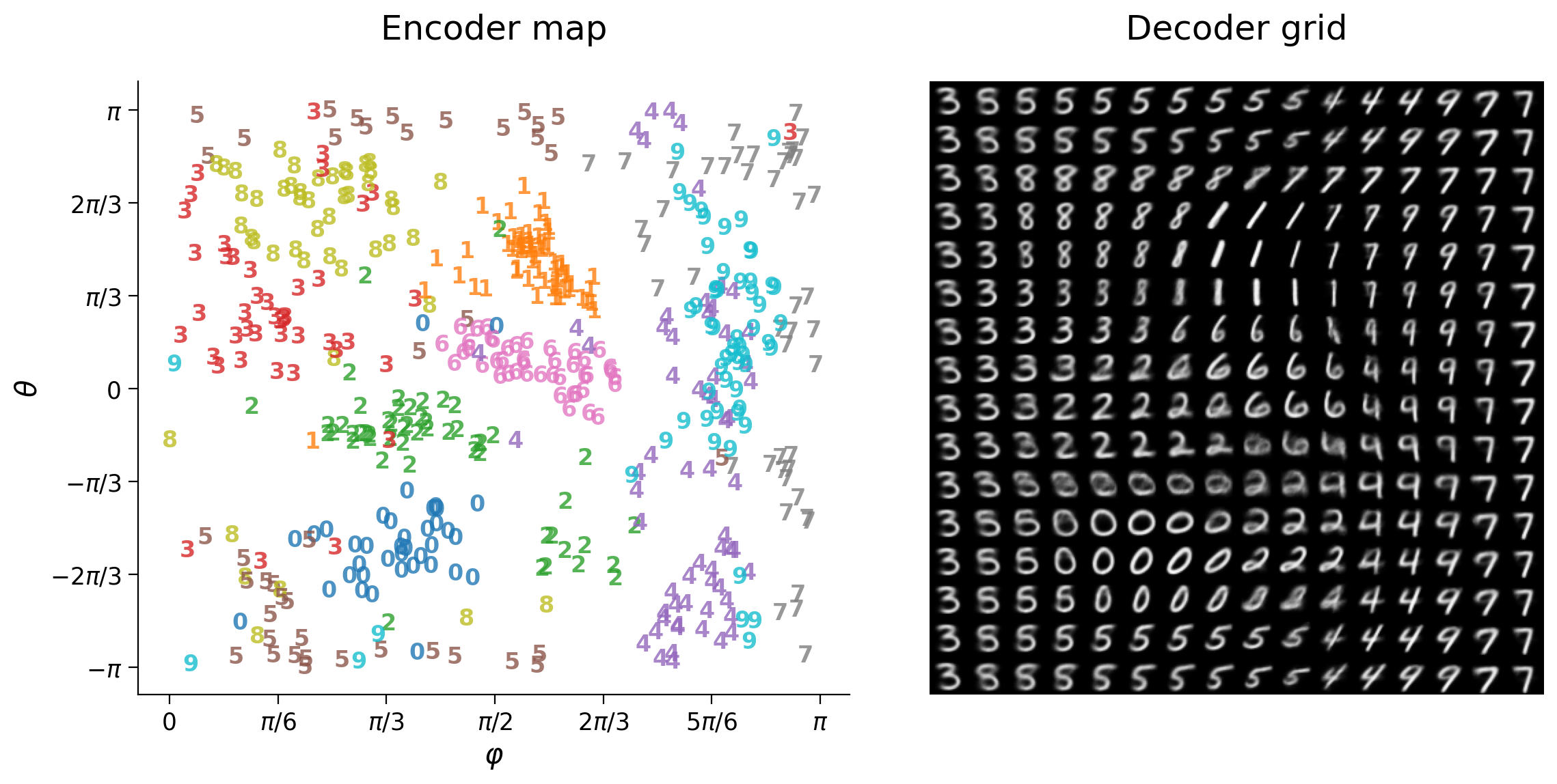
Section 3: Applications of autoencoders
Application 1 - Image noise
Removing noise added to images is often showcased in dimensionality reduction techniques. The tutorial in Dimensionality reduction day illustrated this capability with PCA.
We first observe that autoencoders trained with noise-free images output noise-free images when receiving noisy images as input. However, the reconstructed images will be different from the original images (without noise) since the added noise maps to different coordinates in latent space.
The ability to map noise-free and noisy versions to similar regions in latent space is known as robustness or invariance to noise. How can we build such functionality into the autoencoder?
The solution is to train the autoencoder with noise-free and noisy versions mapping to the noise-free version. A faster alternative is to re-train the autoencoder for few epochs with noisy images. These short training sessions fine-tune the weights to map noisy images to their noise-free versions from similar latent space coordinates.
Let’s start by resetting to the reference state of the autoencoder.
Instructions:
Please execute the cells below
reset_checkpoint(model, optimizer, checkpoint)

with torch.no_grad():
  latent_test_ref = encoder(input_test)
Reconstructions before fine-tuning
Let’s verify that an autoencoder trained on clean images will output clean images from noisy inputs. We visualize this by plotting three rows:
Top row with noisy images inputs
Middle row with reconstructions of noisy images
Bottom row with reconstructions of the original images (noise-free)

The bottom row helps identify samples with reconstruction issues before adding noise. This row shows the baseline reconstruction quality for these samples rather than the original images. (Why?)
Instructions:
Please execute the cell(s) below
noise_factor = 0.4

input_train_noisy = (input_train
                     + noise_factor * np.random.normal(size=input_train.shape))
input_train_noisy = np.clip(input_train_noisy, input_train.min(),
                            input_train.max(), dtype=np.float32)

input_test_noisy = (input_test
                    + noise_factor * np.random.normal(size=input_test.shape))
input_test_noisy = np.clip(input_test_noisy, input_test.min(),
                           input_test.max(), dtype=np.float32)
with torch.no_grad():
  output_test_noisy = model(input_test_noisy)
  latent_test_noisy = encoder(input_test_noisy)
  output_test = model(input_test)

plot_row([input_test_noisy[test_selected_idx],
          output_test_noisy[test_selected_idx],
          output_test[test_selected_idx]], image_shape=image_shape)


Latent space before fine-tuning
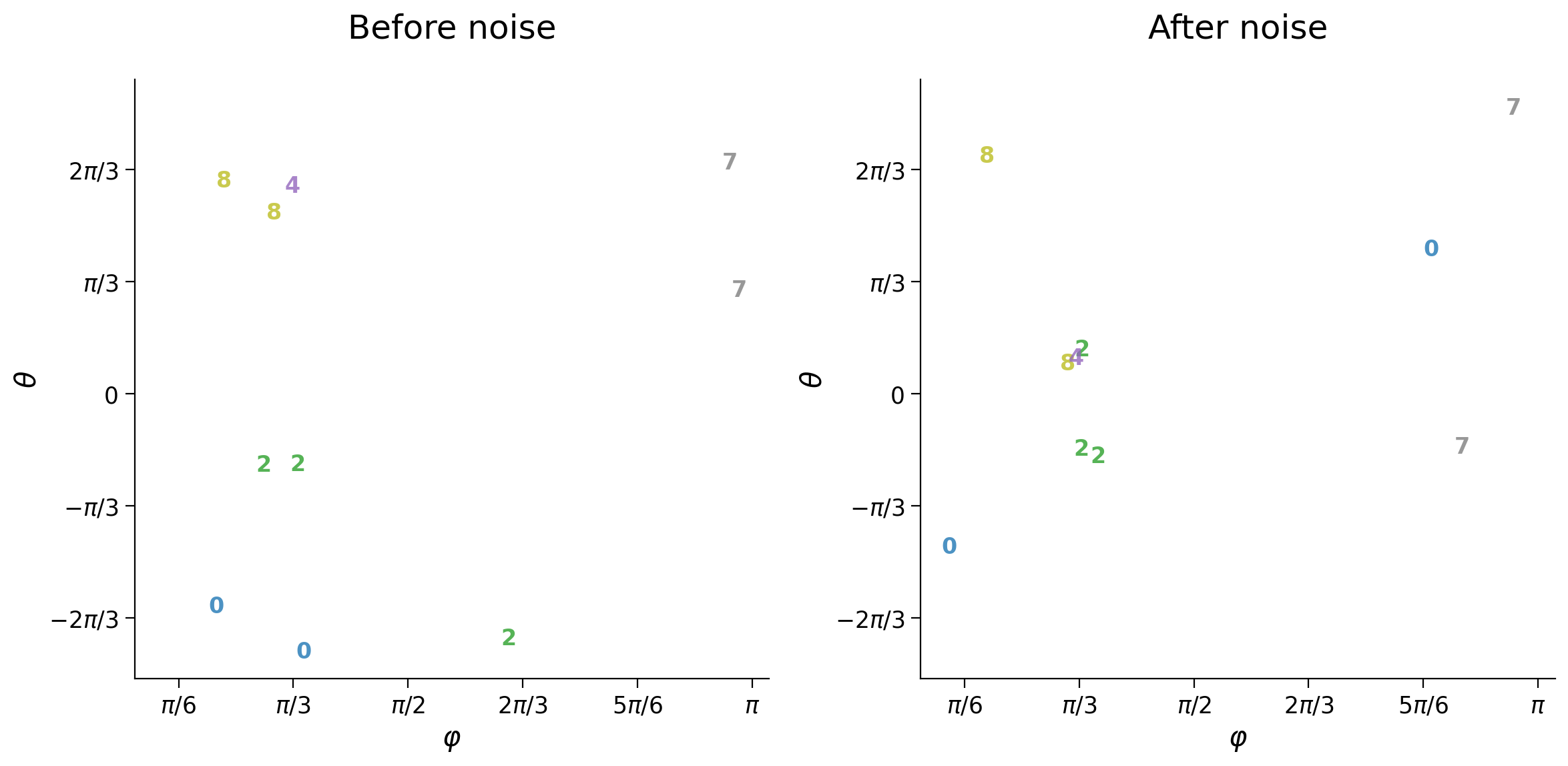
We investigate the origin of reconstruction errors by looking at how adding noise to input affects latent space coordinates. The decoder interprets significant coordinate changes as different digits.
The function plot_latent_ab compares latent space coordinates for the same set of samples between two conditions. Here, we display coordinates for the ten samples from the previous cell before and after adding noise:
The left plot shows the coordinates of the original samples (noise-free)
The plot on the right shows the new coordinates after adding noise
Instructions:
Please execute the cell below
plot_latent_ab(latent_test, latent_test_noisy, y_test, test_selected_idx,
               title_a='Before noise', title_b='After noise', s2=s2)
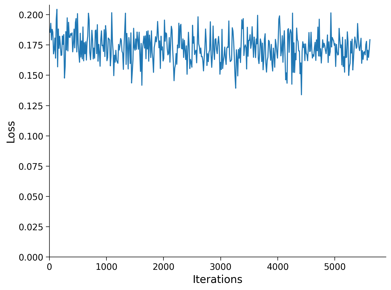
Fine-tuning the autoencoder with noisy images
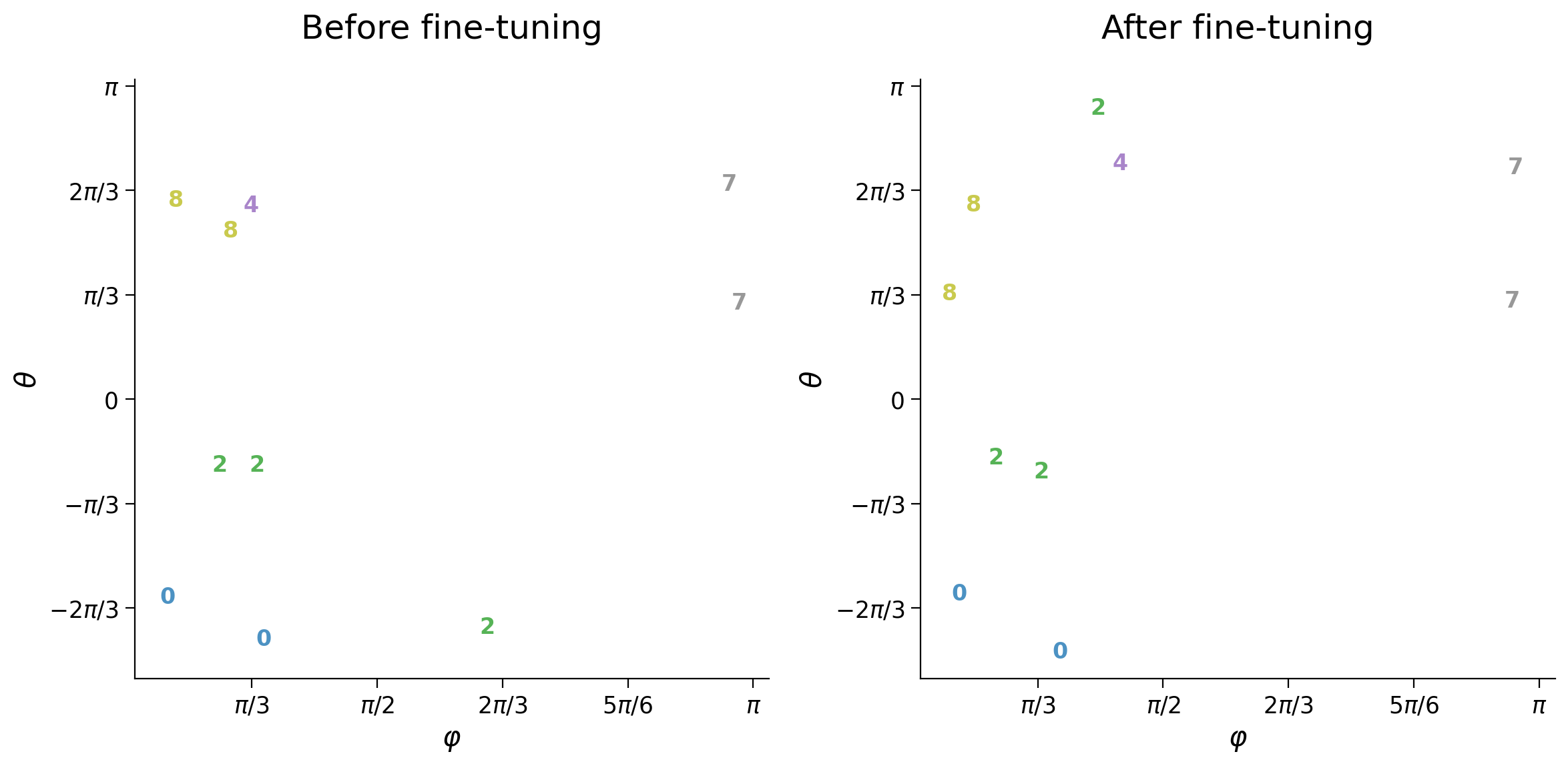
Let’s re-train the autoencoder with noisy images on the input and original (noise-free) images on the output, and regenerate the previous plots.
We now see that both noisy and noise-free images match similar locations in latent space. The network denoises the input with a latent-space representation that is more robust to noise.
Instructions:
Please execute the cell(s) below
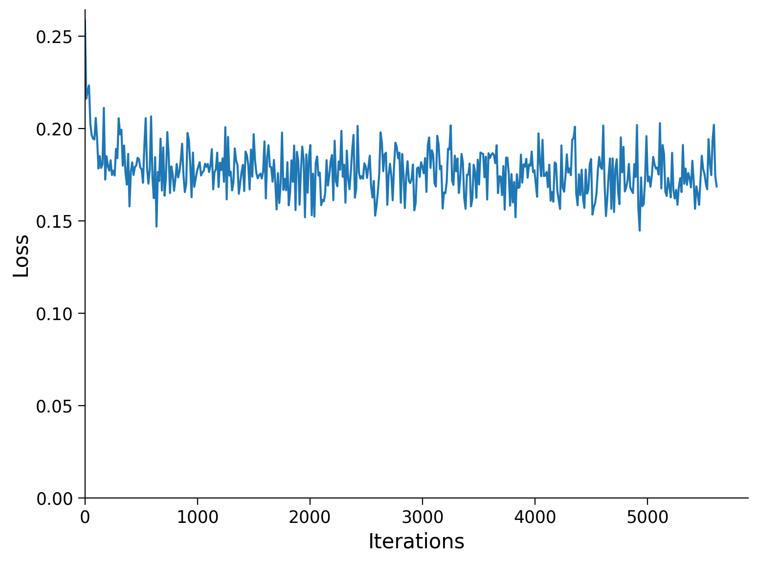
n_epochs = 3
batch_size = 32

model.train()

runSGD(model, input_train_noisy, input_test_noisy,
       out_train=input_train, out_test=input_test,
       n_epochs=n_epochs, batch_size=batch_size)
Epoch Loss train Loss test
1/3 0.1751 0.1759
2/3 0.1742 0.1754
3/3 0.1745 0.1752
with torch.no_grad():
  output_test_noisy = model(input_test_noisy)
  latent_test_noisy = encoder(input_test_noisy)
  output_test = model(input_test)

plot_row([input_test_noisy[test_selected_idx],
          output_test_noisy[test_selected_idx],
          output_test[test_selected_idx]], image_shape=image_shape)

plot_latent_ab(latent_test, latent_test_noisy, y_test, test_selected_idx,
               title_a='Before fine-tuning',
               title_b='After fine-tuning', s2=s2)


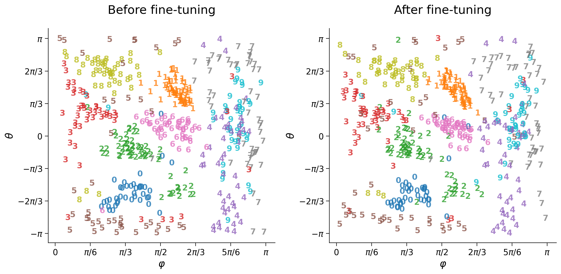
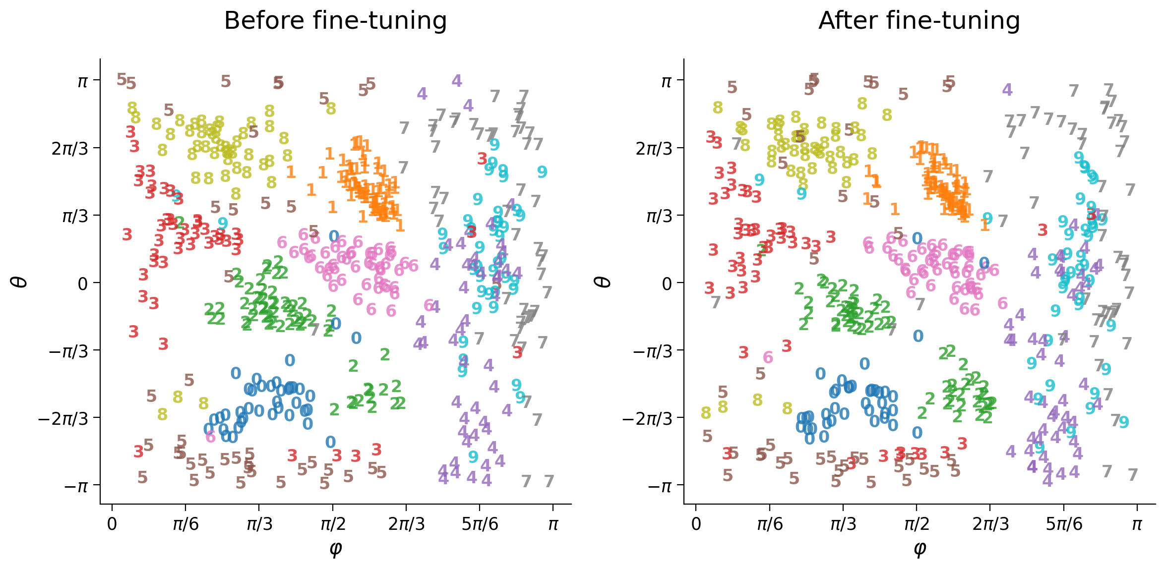
Global latent space shift
The new latent space representation is more robust to noise and may result in a better internal representation of the dataset. We verify this by inspecting the latent space with clean images before and after fine-tuning with noisy images.
Fine-tuning the network with noisy images causes a domain shift in the dataset, i.e., a change in the distribution of images since the dataset was initially composed of noise-free images. Depending on the task and the extent of changes during re-train, (number of epochs, optimizer characteristics, etc.), the new latent space representation may become less well adapted to the original data as a side-effect. How could we address domain shift and improve both noisy and noise-free images?
Instructions:
Please execute the cell(s) below
with torch.no_grad():
  latent_test = encoder(input_test)

plot_latent_ab(latent_test_ref, latent_test, y_test, test_subset_idx,
               title_a='Before fine-tuning',
               title_b='After fine-tuning', s2=s2)
Application 2 - Image occlusion
We now investigate the effects of image occlusion. Drawing from the previous exercise, we expect the autoencoder to reconstruct complete images since the train set does not contain occluded images (right?).
We visualize this by plotting three rows:
Top row with occluded images
Middle row with reconstructions of occluded images
Bottom row with reconstructions of the original images

Similarly, we investigate the source of this issue by looking at the representation of partial images in latent space and how it adjusts after fine-tuning.
Instructions:
Please execute the cell(s) below
reset_checkpoint(model, optimizer, checkpoint)

with torch.no_grad():
  latent_test_ref = encoder(input_test)
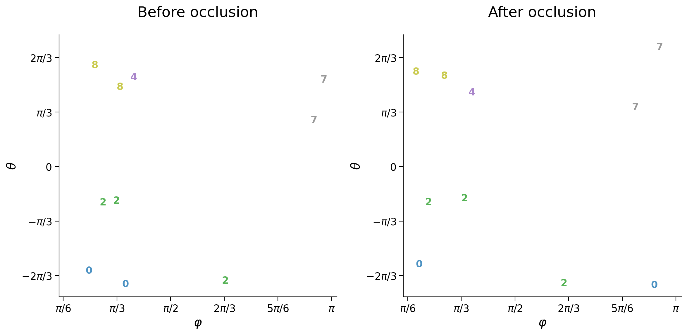
Before fine-tuning
Instructions:
Please execute the cell(s) below
input_train_mask = image_occlusion(input_train, image_shape=image_shape)
input_test_mask = image_occlusion(input_test, image_shape=image_shape)
with torch.no_grad():
  output_test_mask = model(input_test_mask)
  latent_test_mask = encoder(input_test_mask)
  output_test = model(input_test)

plot_row([input_test_mask[test_selected_idx],
          output_test_mask[test_selected_idx],
          output_test[test_selected_idx]], image_shape=image_shape)

plot_latent_ab(latent_test, latent_test_mask, y_test, test_selected_idx,
               title_a='Before occlusion', title_b='After occlusion', s2=s2)


After fine-tuning
n_epochs = 3
batch_size = 32

model.train()

runSGD(model, input_train_mask, input_test_mask,
       out_train=input_train, out_test=input_test,
       n_epochs=n_epochs, batch_size=batch_size)
Epoch Loss train Loss test
1/3 0.1725 0.1733
2/3 0.1708 0.1719
3/3 0.1706 0.1719
with torch.no_grad():
  output_test_mask = model(input_test_mask)
  latent_test_mask = encoder(input_test_mask)
  output_test = model(input_test)

plot_row([input_test_mask[test_selected_idx],
          output_test_mask[test_selected_idx],
          output_test[test_selected_idx]], image_shape=image_shape)

plot_latent_ab(latent_test, latent_test_mask, y_test, test_selected_idx,
               title_a='Before fine-tuning',
               title_b='After fine-tuning', s2=s2)


with torch.no_grad():
  latent_test = encoder(input_test)

plot_latent_ab(latent_test_ref, latent_test, y_test, test_subset_idx,
               title_a='Before fine-tuning',
               title_b='After fine-tuning', s2=s2)
Application 3 - Image rotation
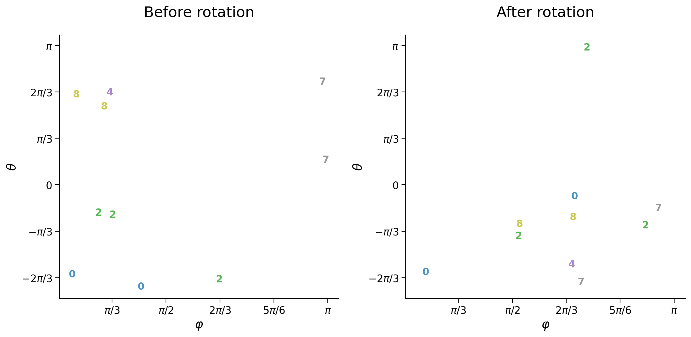
Finally, we look at the effect of image rotation in latent space coordinates. This task is arguably more challenging since it may require a complete re-write of image reconstruction.
We visualize this by plotting three rows:
Top row with rotated images
Middle row with reconstructions of rotated images
Bottom row with reconstructions of the original images

We investigate the source of this issue by looking at the representation of rotated images in latent space and how it adjusts after fine-tuning.
Instructions:
Please execute the cell(s) below
reset_checkpoint(model, optimizer, checkpoint)

with torch.no_grad():
  latent_test_ref = encoder(input_test)
Before fine-tuning
Instructions:
Please execute the cell(s) below
input_train_rotation = image_rotation(input_train, 90, image_shape=image_shape)
input_test_rotation = image_rotation(input_test, 90, image_shape=image_shape)
with torch.no_grad():
  output_test_rotation = model(input_test_rotation)
  latent_test_rotation = encoder(input_test_rotation)
  output_test = model(input_test)

plot_row([input_test_rotation[test_selected_idx],
          output_test_rotation[test_selected_idx],
          output_test[test_selected_idx]], image_shape=image_shape)

plot_latent_ab(latent_test, latent_test_rotation, y_test, test_selected_idx,
               title_a='Before rotation', title_b='After rotation', s2=s2)


After fine-tuning
Instructions:
Please execute the cell(s) below
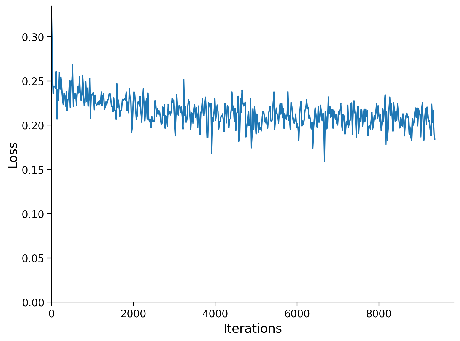
n_epochs = 5
batch_size = 32

model.train()

runSGD(model, input_train_rotation, input_test_rotation,
       out_train=input_train, out_test=input_test,
       n_epochs=n_epochs, batch_size=batch_size)
Epoch Loss train Loss test
1/5 0.2191 0.2191
2/5 0.2122 0.2128
3/5 0.2097 0.2109
4/5 0.2053 0.2065
5/5 0.2046 0.2055
with torch.no_grad():
output_test_rotation = model(input_test_rotation)
latent_test_rotation = encoder(input_test_rotation)
output_test = model(input_test)
plot_row([input_test_rotation[test_selected_idx],
output_test_rotation[test_selected_idx],
output_test[test_selected_idx]], image_shape=image_shape)
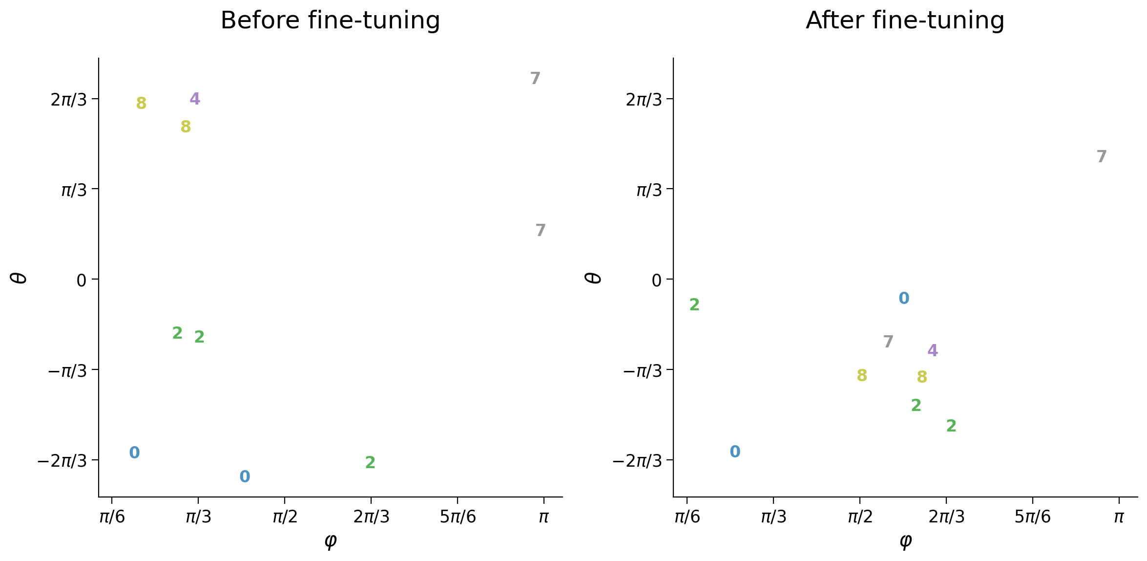
plot_latent_ab(latent_test, latent_test_rotation, y_test, test_selected_idx,
title_a='Before fine-tuning',
title_b='After fine-tuning', s2=s2)


with torch.no_grad():
  latent_test = encoder(input_test)

plot_latent_ab(latent_test_ref, latent_test, y_test, test_subset_idx,
               title_a='Before fine-tuning',
               title_b='After fine-tuning', s2=s2)
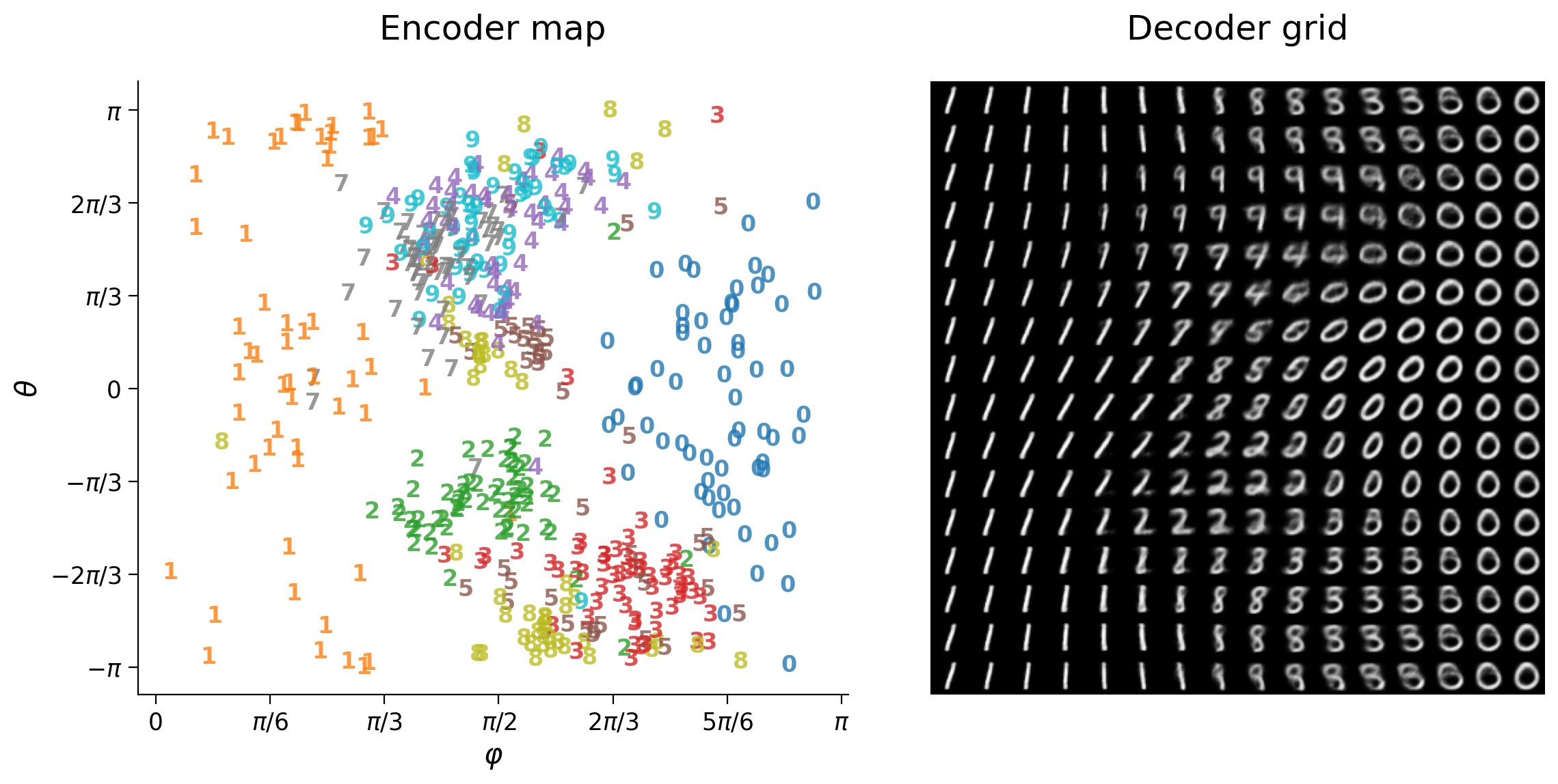
Application 4 - What would digit “6” look like if we had never seen it before?
Before we start melting our brains with such an impossible task, let’s just ask the autoencoder to do it!
We train the autoencoder from scratch without digit class 6 and visualize reconstructions from digit 6.
Instructions:
Please execute the cell(s) below
model = AutoencoderClass(s2=s2)
optimizer = optim.Adam(model.parameters())

encoder = model.encoder
decoder = model.decoder
missing = 6

my_input_train = input_train[y_train != missing]
my_input_test = input_test[y_test != missing]
my_y_test = y_test[y_test != missing]
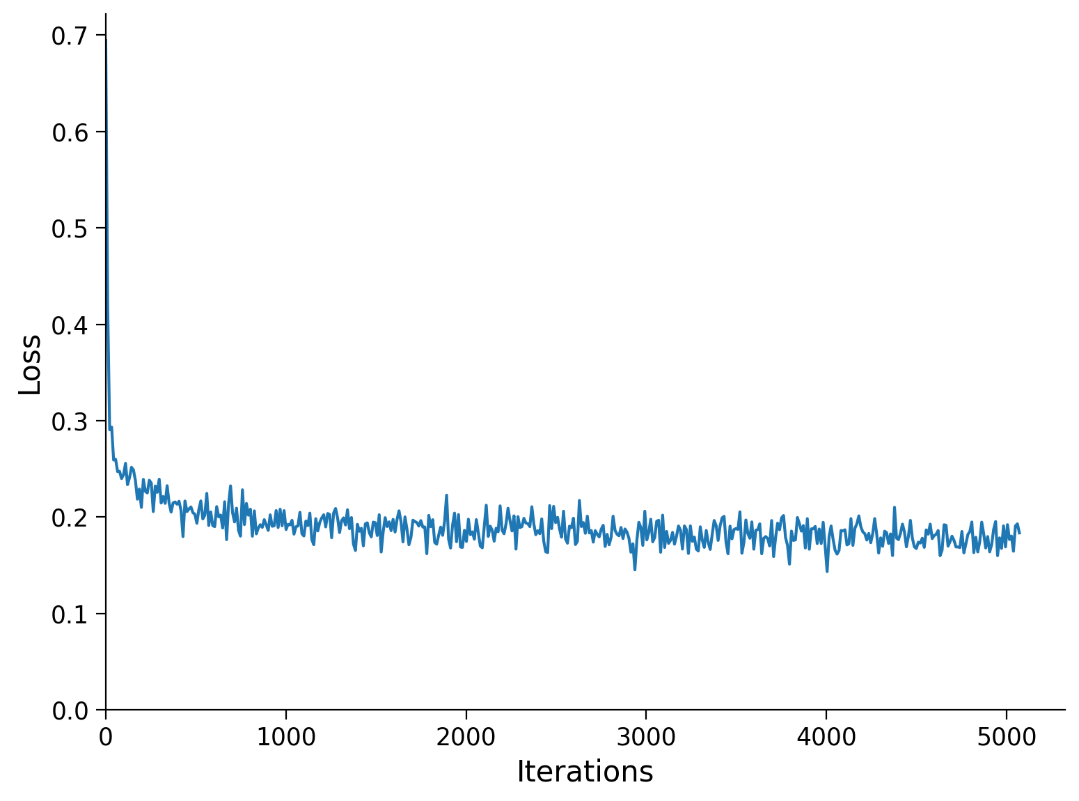
n_epochs = 3
batch_size = 32

runSGD(model, my_input_train, my_input_test,
       n_epochs=n_epochs, batch_size=batch_size)

with torch.no_grad():
  output_test = model(input_test)
  my_latent_test = encoder(my_input_test)
Epoch Loss train Loss test
1/3 0.1881 0.1867
2/3 0.1817 0.1805
3/3 0.1781 0.1774
plot_row([input_test[y_test == 6], output_test[y_test == 6]],
         image_shape=image_shape)

plot_latent_generative(my_latent_test, my_y_test, decoder,
                       image_shape=image_shape, s2=s2)


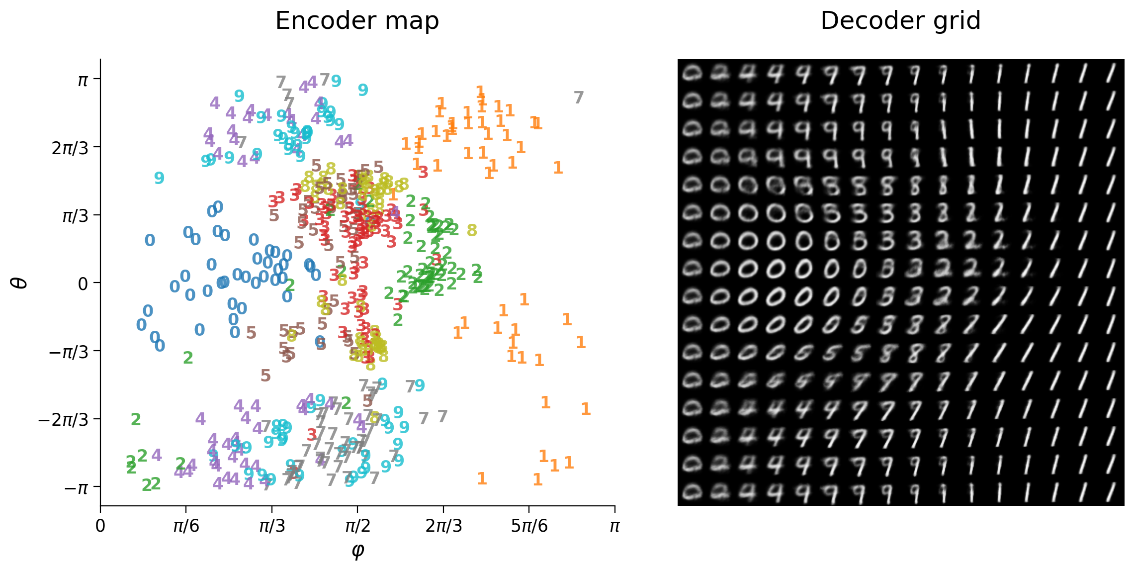
Coding Exercise 1: Removing the most dominant digit classes
Digit classes 0 and 1 are dominant in the sense that these occupy large areas of the decoder grid, compared to other digit classes that occupy very little generative space.
How will latent space change when removing the two most dominant digit classes? Will latent space re-distribute evenly among remaining classes or choose another two dominant classes?
Instructions:
Please execute the cell(s) below
The intersection of two boolean arrays by condition is specified as
x[(cond_a)&(cond_b)]
model = AutoencoderClass(s2=s2)
optimizer = optim.Adam(model.parameters())

encoder = model.encoder
decoder = model.decoder
missing_a = 1
missing_b = 0
#####################################################################
# Fill in missing code (...),
# then remove or comment the line below to test your function
raise NotImplementedError("Complete the code elements below!")
#####################################################################
# input train data
my_input_train = ...
# input test data
my_input_test = ...
# model
my_y_test = ...

print(my_input_train.shape)
print(my_input_test.shape)
print(my_y_test.shape)
SAMPLE OUTPUT
torch.Size([47335, 784])
torch.Size([7885, 784])
torch.Size([7885])
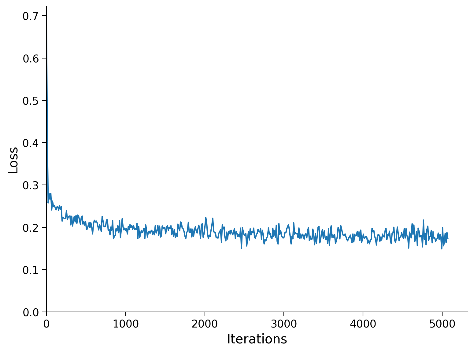
n_epochs = 3
batch_size = 32

runSGD(model, my_input_train, my_input_test,
       n_epochs=n_epochs, batch_size=batch_size)

with torch.no_grad():
  output_test = model(input_test)
  my_latent_test = encoder(my_input_test)
Epoch Loss train Loss test
1/3 0.1894 0.1882
2/3 0.1811 0.1802
3/3 0.1775 0.1765
plot_row([input_test[y_test == missing_a], output_test[y_test == missing_a]],
         image_shape=image_shape)

plot_row([input_test[y_test == missing_b], output_test[y_test == missing_b]],
         image_shape=image_shape)

plot_latent_generative(my_latent_test, my_y_test, decoder,
                       image_shape=image_shape, s2=s2)


Submit your feedback
# @title Submit your feedback
content_review(f"{feedback_prefix}_Removing_the_most_dominant_class_Exercise")
Section 4: ANNs? Same but different!
“Same same but different” is an expression used in some parts of Asia to express differences between supposedly similar subjects. In this exercise, we investigate a fundamental difference in how fully-connected ANNs process visual information compared to human vision.
The previous exercises showed ANN autoencoder performing cognitive tasks with relative ease. However, there is a crucial aspect of ANN processing already encoded in the vectorization of images. This network architecture completely ignores the relative position of pixels. To illustrate this, we show that learning proceeds just as well with shuffled pixel locations.
First, we obtain a reversible shuffle map stored in shuffle_image_idx used to shuffle image pixels randomly.
![]()
The unshuffled image set input_shuffle is recovered as follows:
input_shuffle[:, shuffle_rev_image_idx]]
First, we set up the reversible shuffle map and visualize a few images with shuffled and unshuffled pixels, followed by their noisy versions.
Instructions:
Please execute the cell(s) below
# create forward and reverse indexes for pixel shuffling
shuffle_image_idx = np.arange(input_size)
shuffle_rev_image_idx = np.empty_like(shuffle_image_idx)

# shuffle pixel location
np.random.shuffle(shuffle_image_idx)

# store reverse locations
for pos_idx, pos in enumerate(shuffle_image_idx):
  shuffle_rev_image_idx[pos] = pos_idx

# shuffle train and test sets
input_train_shuffle = input_train[:, shuffle_image_idx]
input_test_shuffle = input_test[:, shuffle_image_idx]

input_train_shuffle_noisy = input_train_noisy[:, shuffle_image_idx]
input_test_shuffle_noisy = input_test_noisy[:, shuffle_image_idx]

# show samples with shuffled pixels
plot_row([input_test_shuffle,
          input_test_shuffle[:, shuffle_rev_image_idx]],
         image_shape=image_shape)


# show noisy samples with shuffled pixels
plot_row([input_train_shuffle_noisy[test_selected_idx],
          input_train_shuffle_noisy[:, shuffle_rev_image_idx][test_selected_idx]],
         image_shape=image_shape)


We initialize and train the network in the denoising task with shuffled pixels.
Instructions:
Please execute the cell below
model = AutoencoderClass(s2=s2)

encoder = model.encoder
decoder = model.decoder

n_epochs = 3
batch_size = 32

# train the model to denoise shuffled images
runSGD(model, input_train_shuffle_noisy, input_test_shuffle_noisy,
       out_train=input_train_shuffle, out_test=input_test_shuffle,
       n_epochs=n_epochs, batch_size=batch_size)
Epoch Loss train Loss test
1/3 0.2014 0.2011
2/3 0.1895 0.1887
3/3 0.1844 0.1842
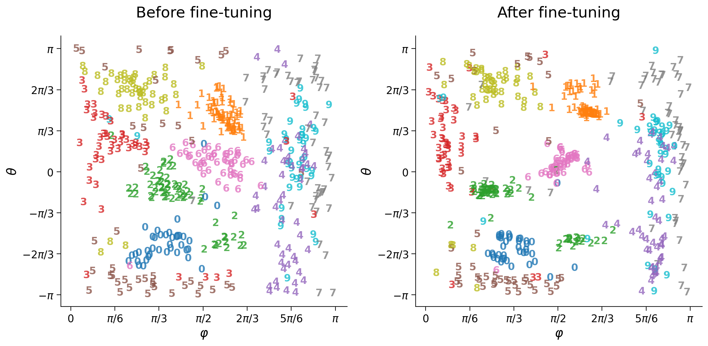
Finally, visualize reconstructions and latent space representation with the trained model.
We visualize reconstructions by plotting three rows:
Top row with shuffled noisy images
Middle row with reconstructions of shuffled denoised images
Bottom row with unshuffled reconstructions of denoised images

We obtain the same organization in the encoder map as before. Sharing similar internal representations confirms the network to ignore the relative position of pixels. The decoder grid is different than before since it generates shuffled images.
Instructions:
Please execute the cell below
with torch.no_grad():
  latent_test_shuffle_noisy = encoder(input_test_shuffle_noisy)
  output_test_shuffle_noisy = model(input_test_shuffle_noisy)

plot_row([input_test_shuffle_noisy[test_selected_idx],
          output_test_shuffle_noisy[test_selected_idx],
          output_test_shuffle_noisy[:, shuffle_rev_image_idx][test_selected_idx]],
         image_shape=image_shape)

plot_latent_generative(latent_test_shuffle_noisy, y_test, decoder,
                       image_shape=image_shape, s2=s2)


Summary
Hooray! You have finished the last Tutorial of NMA 2020!
We hope you’ve enjoyed these tutorials and learned about the usefulness of autoencoders to model rich and non-linear representations of data. We hope you may find them useful in your research, perhaps to model certain aspects of cognition or even extend them to biologically plausible architectures - autoencoders of spiking neurons, anyone?
These are the key take away messages from these tutorials:
Autoencoders trained in learning by doing tasks such as compression/decompression, removing noise, etc. can uncover rich lower-dimensional structure embedded in structured images and other cognitively relevant data.
The data domain seen during training imprints a “cognitive bias” - you only see what you expect to see, which can only be similar to what you saw before.
Such bias is related to the concept What you see is all there is coined by Daniel Kahneman in psychology.
For additional applications of autoencoders to neuroscience, check the spike sorting application in the outro video, and also see here how to replicate the input-output relationship of real networks of neurons with autoencoders.
Video 2: Wrap-up
Submit your feedback
# @title Submit your feedback
content_review(f"{feedback_prefix}_WrapUp_Video")